Plotting Functions on Ordinals
Let’s say we’ve defined a function f from ordinals to ordinals and want to plot it like we might plot a function from integers to integers. We want to line up our ordinals on the x- and y-axes, and plot a point at (x, f(x)) for each ordinal x. Well where should we actually put those ordinals on the axes? This simple question is the topic of this post.

When we’re plotting functions from integers to integers, we simply space out all integers evenly on the axes. This clearly won’t work for our case because we’ll only be able to fit the first ω ordinals. What we need is literally a function t from ordinals to the (positive) real number line telling us where to put tick marks on the axes. This is akin to the trick people use to plot really big finite numbers: use a log-log plot to squish the really big numbers into a manageable and visually appealing domain using t(x) := log(x).

We retrict our attention here to just the ordinals up to ε₀ because they are easy to represent in code, so we seek a function t : ε₀ → ℝ⁺ with a few desiderata:
-
t should be strictly increasing.
-
t should be continuous, i.e. the limit of t mapped over any infinite sequence should equal t applied to the limit of the sequence. For example, the sequence [t(1), t(2), t(3), …] should approach t(ω).
-
t(ω) = 1, t(ω^ω) = 2, t(ω^ω^ω) = 3, …
Desideratum 1 is something we obviously want for our plotting purposes so ticks don’t overlap and they increase from left to right, but even that is tricky to satisfy. It seems like it should be easy because ε₀ is countable and the reals aren’t, but there are just so many ordinals to squeeze onto the line. Desideratum 2 is also very natural for the aesthetics of plotting, but once again is trickier to accomplish than it seems. The last desideratum is actually quite easy to accomplish once we have the first two, but has some interesting implictions. Since t approximates the height of the power tower defining an ordinal, it acts as a super-logarithm (slog; an inverse of tetration) in base ω. Also, combined with desideratum 2, we see that t(ε₀) = t(ω^ω^…) = ∞, so our ticks will fill the axes and we’ll have a sort of “slog-slog” plot.

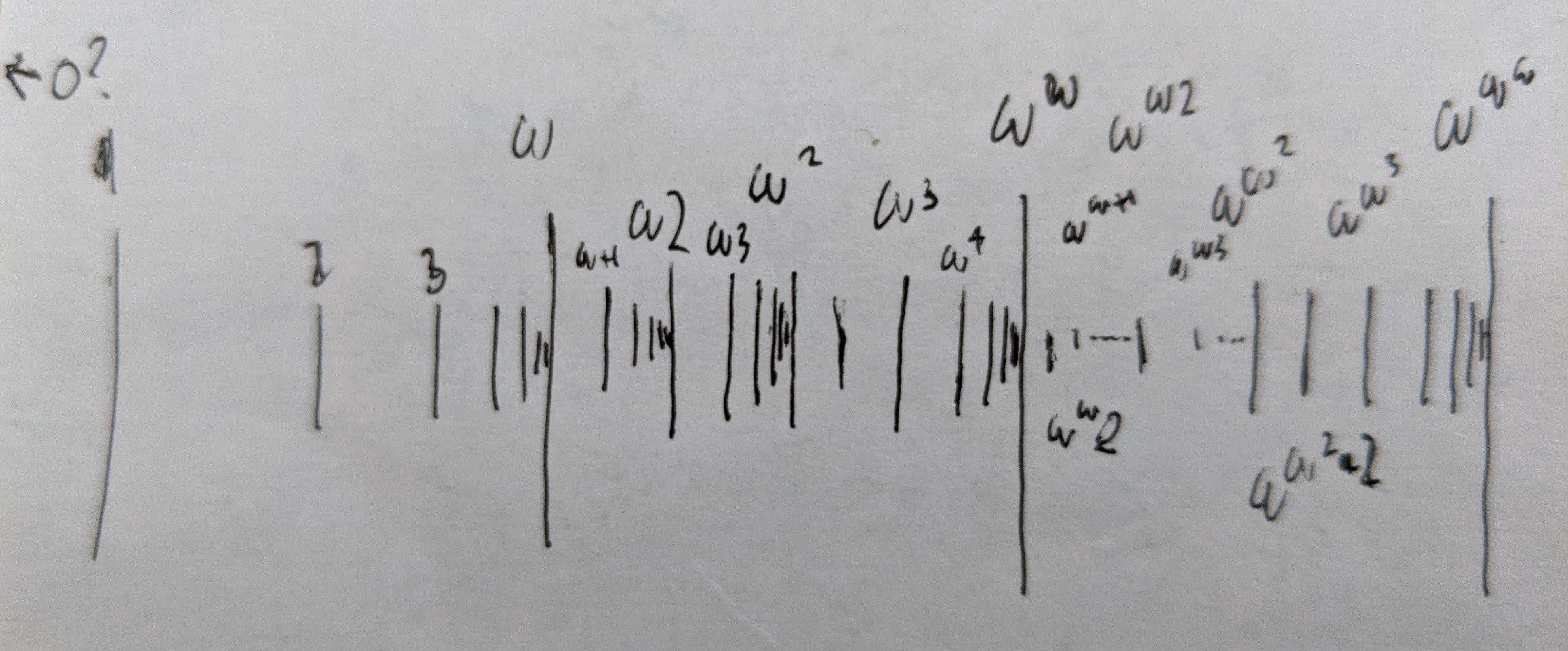
If we draw the kind of function we have in mind, it seems simple enough. For every inifinite sequence like 1, 2, 3, …, we can place each ordinal somewhere between its predecessor and the limit of the sequence. For example, t(3) is about halfway between t(2) and t(ω). But how can we formalize this in a function? After a lot of head-scratching and googling, one might come across a succinct representation of ordinal trees using balanced parentheses (BP) that we can use for desideratum 1. The first step of the conversion from ordinals to BP is to convert to Cantor Normal Form, as in the image above. In short, all ordinals up to ε₀ can be represented as a sort of polynomial in base ω where all exponents are sorted and are themselves in Cantor Normal Form:

For example, ω+3 = ω^ω^0+ω^0+ω^0+ω^0. Such a polynomial can be interpreted as an ordinal tree where the value of each node is the sum of ω to the power of the values of its child nodes:

This tree can be represented succintly as a string of balanced parentheses. Since eventually we’ll have unbalanced parentheses, let’s use “\” and “/” as open and close parens to protect our eyes:

So for example, BP(ω+3) = BP(ω^ω^0+ω^0+ω^0+ω^0) = \//\/\/\/. Now this can be converted to a bitstring by replacing “\”s by 1s and “/”s by 0s, and prepending a “0.”, which can then be interpreted as a real number:
ω+3 → \//\/\/\/ → 0.1100101010 → ~0.79102
It turns out that the above satisfies desideratum 1 because the lexicographic order of the BP-strings respects the order of the ordinals. Since all ordinals get mapped into the 0–1 interval, we can also easily satisfy desideratum 3 by stretching the results to ℝ⁺ with the function s(x) = -log₂(1-x):
ω+3 → \//\/\/\/ → 0.1100101010 → ~0.79102→ ~2.25853
We’re almost there. There’s just one nasty problem with this. If we plot it, we can see that desideratum 2 isn’t met: the ticks for 1, 2, 3, … don’t reach all the way to the tick for ω:

This is because our BP function is defined for ordinal trees in general, including “illegal” unsorted ones that don’t satisfy the i < j ⇒ αᵢ ≥ αⱼ condition, like 1+ω. The current function leaves room for 1+ω at \/\// between all natural numbers at (\/)*n and ω at \//.
This can be fixed by removing all redundant closing parentheses. We consider a close paren to be redundant if, were it an open paren, the corresponding ordinal would be illegal. Since it must be a close paren, we can just omit it and still be able to recover the ordinal from the unbalanced parentheses (UP). So for example, 2 is represented as \/\/, but that last close paren is redundant because UP strings starting with \/\ can only correspond to illegal ordinals like 1+ω. Our updated UP function maps 2 to \/\, 3 to \/\, and natural numbers n to \/()*(n-1).
ω+3 → \//\/\ → 0.11001011 → ~0.79297→ ~2.27208
Now the sequence [t(1), t(2), t(3), …] is [\/, \/\, \/\, …] which is [0.10, 0.101, 0.1011, …], which approaches 0.1100 = t(ω) as desired.

This UP function can be implemented by keeping track of bounds on recursed arguments and omitting closing parentheses when that bound is reached:

To show off our work, we can now plot functions from ordinals to ordinals like f(x) := x*x:

The repo can be found here: https://github.com/asvarga/ordinals-python